Internal structure of Arrow objects
Source:vignettes/developers/data_object_layout.Rmd
data_object_layout.RmdThis article describes the internal structure of Arrow data objects. Users of the arrow R package will not generally need to understand the internal structure of Arrow data objects. We include it here to help orient those R users and Arrow developers who wish to understand the Arrow specification. This article provides a deeper dive into some of the topics described in the data objects article, and is intended mostly for developers. It is not necessary knowledge for using the arrow package.
We begin by describing two key concepts:
- Values in an array are stored in one or more buffers. A buffer is a sequential virtual address space (i.e., block of memory) with a given length. Given a pointer specifying the memory address where the buffer starts, you can reach any byte in the buffer with an “offset” value that specifies a location relative to the start of the buffer.
- The physical layout of an array is a term used to describe how data in an array is laid out in memory, without taking into account how that information is interpreted. As an example: a 32-bit signed integer and 32-bit floating point number have the same layout: they are both 32 bits, represented as 4 contiguous bytes in memory. The meaning is different, but the layout is the same.
We can unpack these ideas using a simple array of integer values:
integer_array <- Array$create(c(1L, NA, 2L, 4L, 8L))
integer_array
## Array
## <int32>
## [
## 1,
## null,
## 2,
## 4,
## 8
## ]We can inspect the integer_array$type attribute to see
that the values in the Array are stored as signed 32 bit integers. When
laid out in memory by the Arrow C++ library, an integer array consists
of two pieces of metadata and two buffers that store the data. The
metadata specify the length of the array and a count of the number of
null values, both stored as 64-bit integers. These metadata can be
viewed from R using integer_array$length() and
integer_array$null_count respectively. The number of
buffers associated with an array depends on the exact type of data being
stored. For an integer array there are two: a “validity bitmap buffer”
and a “data value buffer”. Schematically we could depict the array as
follows:
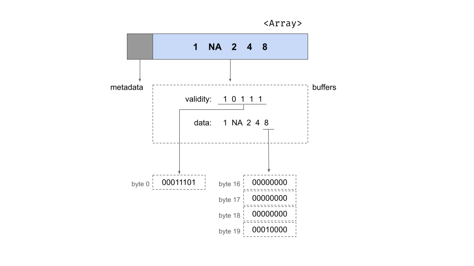
This image shows the array as a rectangle subdivided into two parts, one for the metadata and the other for the buffers. Underneath the rectangle we’ve unpacked the contents of the buffers for you, showing the contents of the two buffers in the area enclosed in a dotted line. At the very bottom of the figure, you can see the contents of specific bytes.
Validity bitmap buffer
The validity bitmap is binary-valued, and contains a 1 whenever the corresponding slot in the array contains a valid, non-null value. At an abstract level we can assume this contains the following five bits:
10111However this is a slight over-simplification for three reasons.
First, because memory is allocated in byte-size units there are three
trailing bits at the end (assumed to be zero), giving us the bitmap
10111000. Second, while we have written this from
left-to-right, this written format is typically presumed to represent big endian format
where the most-significant bit is written first (i.e., to the
lowest-valued memory address). Arrow adopts a little-endian convention,
which would more naturally correspond toa right-to-left ordering when
written in English. To reflect this we write the bits in right-to-left
order: 00011101. Finally, Arrow encourages naturally
aligned data structures in which allocated memory addresses are a
multiple of the data block sizes. Arrow uses 64 byte alignment,
so each data structure must be a multiple of 64 bytes in size. This
design feature exists to allow efficient use of modern hardware, as
discussed in the Arrow
specification. This is what the buffer looks like this in
memory:
| Byte 0 (validity bitmap) | Bytes 1-63 |
|---|---|
00011101 |
0 (padding) |
Data buffer
The data buffer, like the validity bitmap, is padded out to a length of 64 bytes to preserve natural alignment. Here’s the diagram showing the physical layout:
| Bytes 0-3 | Bytes 4-7 | Bytes 8-11 | Bytes 12-15 | Bytes 16-19 | Bytes 20-63 |
|---|---|---|---|---|---|
1 |
unspecified | 2 |
4 |
8 |
unspecified |
Each integer occupies 4 bytes, as per the requirements of a 32-bit signed integer. Notice that the bytes associated with the missing value are left unspecified: space is allocated for the value but those bytes are not filled.
Offset buffer
Some types of Arrow array include a third buffer known as the offset buffer. This is most frequently encountered in the context of string arrays, such as this one:
string_array <- Array$create(c("hello", "amazing", "and", "cruel", "world"))
string_array
## Array
## <string>
## [
## "hello",
## "amazing",
## "and",
## "cruel",
## "world"
## ]Using the same schematic notation as before, this is the structure of the object. It has the same metadata as before but as shown below, there are now three buffers:
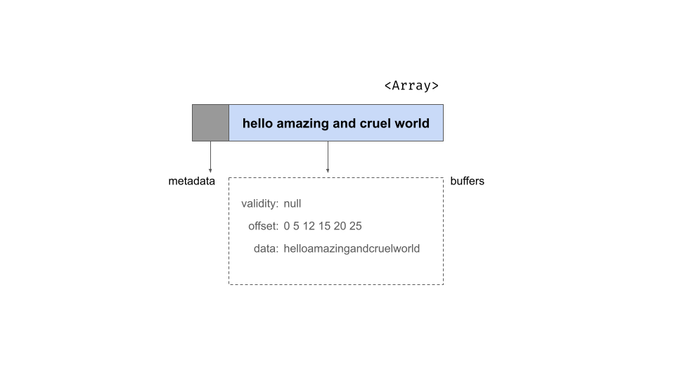
To understand the role of the offset buffer, it helps to note the
format of the data buffer for a string array: it concatenates all
strings end to end in one contiguous section of memory. For the
string_array object, the contents of the data buffer would
look like one long utf8-encoded string:
helloamazingandcruelworldBecause individual strings can be of variable length, the role of the
offset buffer is to specify where the boundaries between the slots are.
The second slot in our array is the string "amazing". If
the positions in the data array are indexed like this
| h | e | l | l | o | a | m | a | z | i | n | g | a | n | d | … |
|---|---|---|---|---|---|---|---|---|---|---|---|---|---|---|---|
| 0 | 1 | 2 | 3 | 4 | 5 | 6 | 7 | 8 | 9 | 10 | 11 | 12 | 13 | 14 | … |
then we can see that the string of interest begins at position 5 and
ends at position 11. The offset buffer consists integers that store
these break point locations. For string_array it might look
like this:
0 5 12 15 20 25The difference between the utf8() data type and the
large_utf8() data type is that these the
utf8() data type stores these as 32-bit integers whereas
the large_utf8() type stores them as 64-bit integers.
Chunked arrays
Arrays are immutable objects: once an Array has been initialized the values it stores cannot be altered. This ensures that multiple entities can safely refer to an Array via pointers, and not run the risk that the values will change. Using immutable Arrays makes it possible for Arrow to avoid unnecessary copies of data objects.
There are limitations to immutable Arrays, most notably when new batches of data arrive. Because an array is immutable, you can’t add the new information to an existing array. The only thing you can do if you don’t want to disturb or copy your existing array is create a new array that contains the new data. Doing that preserves the immutability of arrays and doesn’t lead to any unnecessary copying but now we have a new problem: the data are split across two arrays. Each array contains only one “chunk” of the data. What would be ideal is an abstraction layer that allows us to treat these two Arrays as though they were a single “Array-like” object.
This is the problem that chunked arrays solve. A chunked array is a wrapper around a list of arrays, and allows you to index their contents “as if” they were a single array. Physically, the data are still stored in separate places – each array is one chunk, and these chunks don’t have to be adjacent to each other in memory – but the chunked array provides us will a layer of abstraction that allows us to pretend that they are all one thing.
To illustrate, let’s use the chunked_array()
function:
chunked_string_array <- chunked_array(
  c("hello", "amazing", "and", "cruel", "world"),
  c("I", "love", "you")
)
The chunked_array() function is just a wrapper around
the functionality that ChunkedArray$create() provides.
Let’s take a look at the object:
chunked_string_array## ChunkedArray
## <string>
## [
## [
## "hello",
## "amazing",
## "and",
## "cruel",
## "world"
## ],
## [
## "I",
## "love",
## "you"
## ]
## ]The double bracketing in this output is intended to highlight the “list-like” nature of chunked arrays. There are three separate arrays, wrapped in a container object that is secretly a list of arrays, but allows that list to behave just like a regular one-dimensional data structure. Schematically it looks like this:
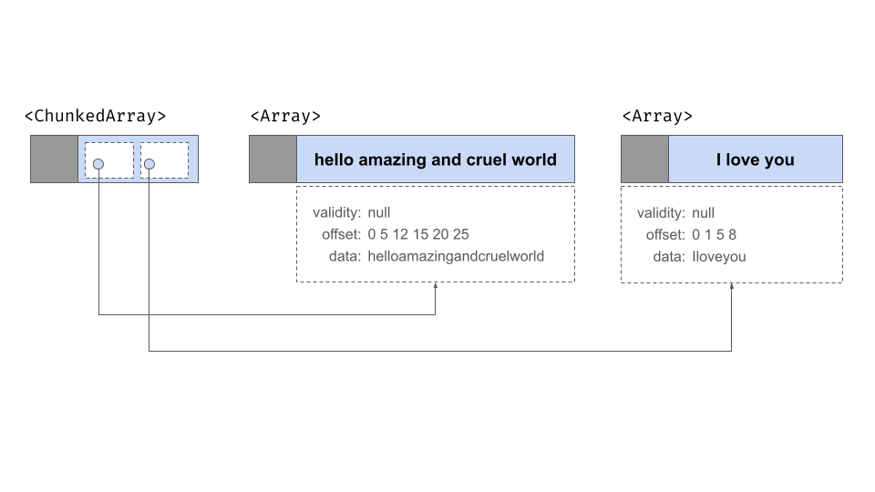
As this figure illustrates, there really are three arrays here, each with its own validity bitmap, offset buffer, and data buffer.
Record batches
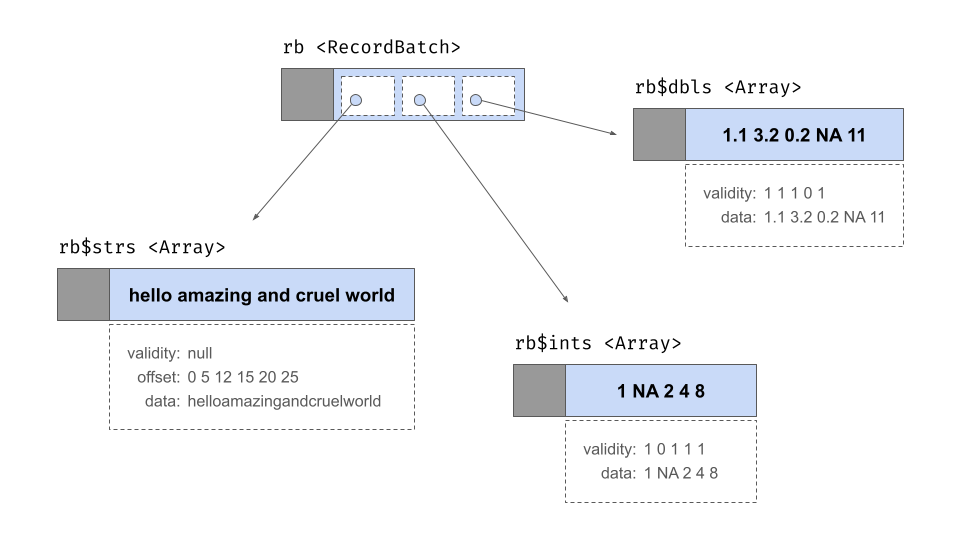
A record batch is table-like data structure comprised of a sequence of arrays. The arrays can be of different types but they must all be the same length. Each array is referred to as one of the “fields” or “columns” of the record batch. Each field must have a (UTF8-encoded) name, and these names form part of the metadata for the record batch. When stored in memory, the record batch does not include physical storage for the values stored in each field: instead it contains pointers to the relevant array objects. It does, however, contain its own validity bitmap.
Here is a record batch containing 5 rows and 3 columns:
rb <- record_batch(
  strs = c("hello", "amazing", "and", "cruel", "world"),
  ints = c(1L, NA, 2L, 4L, 8L),
  dbls = c(1.1, 3.2, 0.2, NA, 11)
)
rb
## RecordBatch
## 5 rows x 3 columns
## $strs <string>
## $ints <int32>
## $dbls <double>At an abstract level the rb object behaves like a two
dimensional structure with rows and columns, but in terms of how it is
represented in memory it is fundamentally a list of arrays as shown
below:
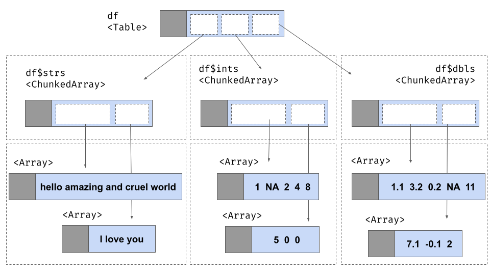
Tables
To deal with situations where a rectangular data set can grow over
time (as more data are added), we need a tabular data structure that is
similar to a record batch with one exception: instead of storing each
column as an array, we now want to store it as a chunked array. This is
what the Table class in arrow does.
To illustrate, suppose we have a second set of data that arrives as a record batch:
new_rb <- record_batch(
  strs = c("I", "love", "you"),
  ints = c(5L, 0L, 0L),
  dbls = c(7.1, -0.1, 2)
)

df <- concat_tables(arrow_table(rb), arrow_table(new_rb))
df
## Table
## 8 rows x 3 columns
## $strs <string>
## $ints <int32>
## $dbls <double>Here is the underlying structure of this Table: